Dixon's Q-test: Detection of a single outlier

Theory

In a set of replicate measurements of a physical or chemical quantity, one or more of the obtained values may differ considerably from the majority of the rest. In this case there is always a strong motivation to eliminate those deviant values and not to include them in any subsequent calculation (e.g. of the mean value and/or of the standard deviation). This is permitted only if the suspect values can be "legitimately" characterized as outliers.

Usually, an outlier is defined as an observation that is generated from a different model or a different distribution than was the main "body" of data. Although this definition implies that an outlier may be found anywhere within the range of observations, it is natural to suspect and examine as possible outliers only the extreme values.

The rejection of suspect observations must be based exclusively on an objective criterion and not on subjective or intuitive grounds. This can be achieved by using statistically sound tests for "the detection of outliers".

The Dixon's Q-test is the simpler test of this type and it is usually the only one described in textbooks of Analytical Chemistry in the chapters of data treatment. This test allows us to examine if one (and only one) observation from a small set of replicate observations (typically 3 to 10) can be "legitimately" rejected or not.

Q-test is based on the statistical distribution of "subrange ratios" of ordered data samples, drawn from the same normal population. Hence, a normal (Gaussian) distribution of data is assumed whenever this test is applied. In case of the detection and rejection of an outier, Q-test cannot be reapplied on the set of the remaining observations.

How the Q-test is applied

The test is very simple and it is applied as follows:

(1) The N values comprising the set of observations under examination are arranged in ascending order:

x₁ < x₂ < . . . < x_N

(2) The statistic experimental Q-value (Q_exp) is calculated. This is a ratio defined as the difference of the suspect value from its nearest one divided by the range of the values (Q: rejection quotient). Thus, for testing x₁ or x_N (as possible outliers) we use the following Q_exp values:

(3) The obtained Q_exp value is compared to a critical Q-value (Q_crit) found in tables. This critical value should correspond to the confidence level (CL) we have decided to run the test (usually: CL=95%).

Note: Q-test is a significance test. For more information on terms and concepts related to significance tests (e.g. null hypothesis, confidence levels, probabilities of type I and type II errors), see the applet: Student's t-test: Comparison of two means.

(4) If Q_exp > Q_crit, then the suspect value can be characterized as an outlier and it can be rejected, if not, the suspect value must be retained and used in all subsequent calculations.

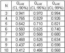
The null hypothesis associated to Q-test is as follows: "There is no a significant difference between the suspect value and the rest of them, any differences must be exclusively attributed to random errors".

A table containing the critical Q values for CL 90%, 95% and 99% and N=3-10 is given below [from: D.B. Rorabacher, Anal. Chem. 63 (1991) 139]

Table of critical values of Q

Typical example

The following replicate observations were obtained during a measurement and they are arranged in ascending order:

4.85, 6.18, 6.28, 6.49, 6.69.

These values can be represented by the following dotplot:

Can we reject observation 4.85 as an outlier at a 95% confidence level?

Answer: The corresponding Q_exp value is: Q_exp = (6.18 - 4.85) / (6.69 - 4.85) = 0.722. Q_exp is greater than Q_crit value (=0.710, at CL:95% for N=5). Therefore we can reject 4.85 and being certain that the probability (p) of erroneous rejection of the null hypothesis (type 1 error) is less than 0.05.

Note: At confidence level 99%, the suspect observation cannot be rejected, hence the probability of erroneous rejection is greater than 0.01.

A general comment on the rejection of outliers

All data rejection tests must be judiciously used. Some statisticians object to the rejection of data from any small size data sample, unless it is solidly known that something went wrong during the corresponding measurement. Other recommend the accommodation of outliers and not their rejection, i.e. they suggest to include deviant values in all subsequent calculations but with reduced statistical weight (Winsorized methods).

It should be also stressed that the use of Q-test is increasingly discouraged in favor of other more robust methods. One such method is the Huber method, which takes into consideration all data present within the set, and not only three as in the case of Q-test.

Applet

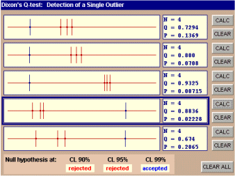
With this applet we can experiment with small data samples (Ν = 3 to 10), which can be easily produced and displayed on each one of the 5 dotplot-areas. By left-clicking the mouse, we can define the position (thus its relative value) of each point (value). After defining 3 to 10 data values, by clicking on the corresponding CALC(: Calculate)-button the most deviant point (suspect value) is automatically located and the corresponding Q_exp is calculated. On the "window" to the right side of the dotplot the number of data-points N comprising the set and the calculated Q_exp is displayed (Q).

The outcome of the test is reported at the lower part of applet working area:

The report (in the present example) is as follows: The null hypothesis is rejected at CL levels 90% and 95%, whereas it is accepted at CL 99%. That means that the probability (p) of type-I error (i.e. erroneous rejection of the null hypothesis) is somewhere between 0.01 and 0.05. This is all the information we can have by using tables of critical values at various confidence levels.

However, this applet can give the actual value of p and this value is shown (as P) in the small window next to the dotplot along with N and Q. For N>4, this calculation is performed by a Monte Carlo procedure, thus it may take some time (typically: 5-10 s) for the final result to appear. More details on how p values are calculated are shown here.

By clicking on the "CLEAR" button the dotplot is cleared and a new data sample can be created and examined as previously described. This applet allows us to create 5 independent dotplots for visual comparison of the obtained results, as it is shown in the screenshot below: