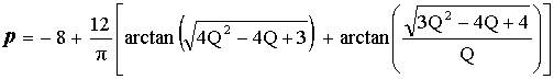
Thus for N = 3 the equation
used is:
Stochastic
(Monte Carlo) estimation of Type I error Probability in Dixon's Q-test
[based on: C. E. EFSTATHIOU: "Estimation of Type I Error Probability from Experimental Dixon's "Q" Parameter on Testing for Outliers within small Size Data Sets", Talanta, 69(5), 1068-1071 (2006)., PDF]
The
traditional way of performing Q-test is based on the use of tabulated critical-Q
values.
However, as it is common to all similarly performed significance tests, this way
cannot provide us with the exact value of type-I error probability (p).
Statistical software packages for performing significance tests have made obsolete the use of tabulated critical values, since their usual outcome is directly the value of p, which is internally computed.
Unfortunately,
in the case of the Q-test, the required mathematics for the calculation of p
are particularly arduous and special numerical integration techniques are
needed.
|
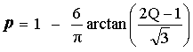
Thus for N = 3 the equation
used is: |
|
| whereas for N = 4 the equation used is (provided that p<0.5, otherwise the Monte Carlo approach is used): |
|
|
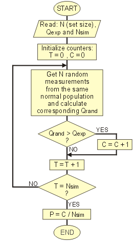
For N > 4 there are no similar analytical expressions, but we can use a simple Monte Carlo approach for the estimation of p. [Note: for a short introduction in Monte Carlo techniques, see applet: Drunken sailor's random walk]. The
algorithm used is as follows: (i)
A set of N random values from the same normally distributed population is
obtained, and the Q-value corresponding to this random set (Qrand) is calculated. (ii)
If this Qrand value
is greater than the input Qexp value,
then
a counter (C) is incremented. (iii)
Steps (i) and (ii) are repeated Nsim times (Nsim : number
of simulations). (iv)
The ratio C / Nsim is the estimated value of p. The
flow-chart of this algorithm is shown to the right: The reasoning behind this algorithm is that all Nsim Qrand–values have been obtained from the same by definition "outliers-free" sets of N random values, since they have been all obtained from the same normal population. Therefore, the fraction of Qrand values greater that the examined Qexp value, represents the probability of normal occurrence Qrand at this range. |
|
Obviously,
a large number Nsim
of simulations is needed
to obtain a reasonably accurate value of p.
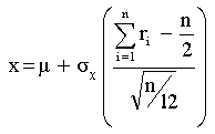
| NOTE: Normally distributed random numbers with mean μ and standard deviation σx can be readily produced by using the equation shown to the right as "random-number generator": |
|
rj is a random number uniformly distributed between 0 and 1. Such random numbers (actually: pseudo-random) are provided by most high-level computer languages. As n increases, the generated x values tend to obtain a normal distribution. Typically, n=12. This "generator" is based on the "Central Limit Theorem" (see applet: Central Limit Theorem)