Least

Least-Squares Polynomial Approximation

Theory

If it is known that the measured quantity y (depended variable) is a linear function of x (independent variable), i.e.

the most probable values of a₀ (intercept) and a₁ (slope) can be estimated from a set of n pairs of experimental data (x₁, y₁), (x₂, y₂)…, (x_n, y_n), where y-values are contaminated with a normally distributed - zero mean random error (e.g. noise, experimental uncertainty). This estimation is known as least-squares linear regression.

Least-squares linear regression is only a partial case of least-squares polynomial regression analysis. By implementing this analysis, it is easy to fit any polynomial of m degree

to experimental data (x₁, y₁), (x₂, y₂)…, (x_n, y_n), (provided that n≥m+1) so that the sum of squared residuals S is minimized:

By obtaining the partial derivatives of S with respect to a₀, a₁, .., a_m and equating these derivatives to zero, the following system of m-equations and m-unknowns (a₀, a₁, .., a_m) is defined:

where:

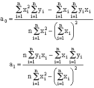
(obviously it is always: s₀ = n)

This system is known a system of normal equations. The set of coefficients: a₀, a₁, …, a_m is the unique solution of this system. For m=1, the familiar expressions used in linear least-square fit are obtained:

Similar (but by far more complicated) expressions are obtained for coefficients of polynomials of higher degrees. Direct use of these expressions for m>1 are almost never used. Instead, the system of normal equations is set and the solution vector of a₀, a₁, …, a_n coefficients is calculated usually with the aid of a computer.

The quality of fit is judged by the coefficient of determination (r²):

is the theoretical y-value corresponding to xi (calculated through the polynomial) and is the mean value of all experimental y-values. It is always 0≤r²≤1. r² =1 indicates a perfect fit (the curve is passing exactly over all data points), whereas r² becomes progressively less than 1 as the scattering of points about the best fitted curve increases. Another measure of the quality of fit is the sum of squared residuals itself and it is obvious that when S=0 we have again a perfect fit.

Applet

This applet demonstrates the general polynomial least-squares regression. The user must click n (n≤200) data points (x, y) in the plot area. While clicking, a line appears which is the graphical presentation of the fitted 1-st degree (linear) equation to data. After clicking several points the user can increase (or decrease) the polynomial degree m (1≤m≤12) by clicking the buttons assigned for this purpose. Remember that it must always be: n≥m+1.

An m-degree polynomial fits exactly to m+1 different data points, e.g. 2 data points always define a line, 3 data points always define a parabola and so on. If n>m+1, the curve drawn describes the m-degree polynomial that fits better to the n data points. This curve is known as approximating curve.

Note that by increasing of the degree m, generally, a better fit is obtained. However, for data points describing a physical phenomenon, polynomial regression with m larger than 1 or 2 is rarely used. It is also interesting that as the degree of polynomial increases, few additional data points can change dramatically many coefficients and the shape of the approximating curve, as well.